NetworkX Graphs¶

The NetworkX library¶

NetworkX is a Python library for creating, manipulating, and displaying mathematical objects called graphs, or networks.

We begin by importing the library:

import networkx as nx

Graphs¶

A graph is a mathematical object that consists of points called nodes together with lines connecting them called edges. Nodes are typically labeled with positive integers, and an edge between two nodes is given by an ordered pair.

G = nx.Graph()
G.add_nodes_from([1,2,3,4,5,6])
G.add_edge(1,4)
nx.draw(G)

In the above code, the function Graph() creates an empty graph object in Python that we can then fill with nodes and edges. Nodes and edges can either be added individually or from a list using different methods.

Below is the graph G generated by the code above.

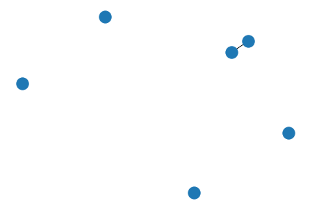
Notice that the layout of the nodes is not ideal, and we do not know which node is which. To make the graph come out looking better, we can add some additional arguments to the draw function.

nx.draw(G, pos=nx.circular_layout(G), with_labels=True)

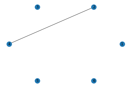
In the above code, the argument pos=nx.circular_layout(G) arranges the nodes in a circle going counterclockwise with the first node on the right. The argument with_labels=True turns on the node labels so we can tell which node is which.

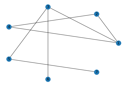
To modify the graph, we do not need to start over from scratch, we can simply add additional nodes and edges using the methods add_node, add_nodes_from, add_edge, and add_edges_from.

G.add_node(7)
G.add_edges_from([(1,2),(1,3),(1,4),(3,5),(3,6),(5,7)])
nx.draw(G, pos=nx.circular_layout(G), with_labels=True)

We can also remove nodes and edges in a similar fashion using the methods remove_node, remove_nodes_from, remove_edge, and remove_edges_from. When removing nodes, any edges containing the removed node will also be removed.

You can take at look at the nodes and edges in your graph at anytime using the nodes and edges methods.

G.nodes()

NodeView((1, 2, 3, 4, 5, 6, 7))

G.edges()

EdgeView([(1, 2), (1, 3), (1, 4), (2, 4), (3, 5), (3, 6), (5, 7)])

The data structure of graph objects is composed of dictionaries with the nodes as keys. If you input the node \(x\), you will get a dictionary containing the nodes connected to \(x\) by an edge. Such nodes are called adjacent or neighbors.

G[1]

AtlasView({2: {}, 3: {}, 4: {}})

The neighborhood of a node is the collection of all its neighbors. For example, the our graph \(G\), the neighborhood of node 1 is the collection of nodes 2, 3, and 4.

The number of nodes in the neighborhood of \(x\) is called the degree of the node \(x\). In our example, the degree of node 1 is 3 since node 1 has 3 neighbors. You can use the degree method to obtain the degree of a node.

G.degree(1)

3

Weighted Edges¶

NetworkX also makes it possible to assign different attributes to each edge, the most common of which are edge weights. An edge weight is a real number associated to an edge, typically representing the importance of the connection between the two corresponding nodes.

A weighted edge between nodes \(x\) and \(y\) with weight \(w\) is represented by the triple \((x,y,w)\).

W = nx.Graph()
W.add_weighted_edges_from([(1,2,1.3),(2,3,1.9),(2,4,0.8),(3,4,2.3)])
nx.draw(W, pos=nx.circular_layout(W), with_labels=True)

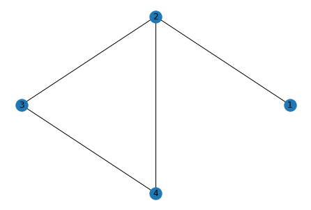
Notice that nx.draw does not draw the edge weights. For that we will need some additional commands.

weights = nx.get_edge_attributes(W,'weight')
nx.draw(W, pos=nx.circular_layout(W), with_labels=True)
nx.draw_networkx_edge_labels(W, pos=nx.circular_layout(W), edge_labels=weights)
plt.show()

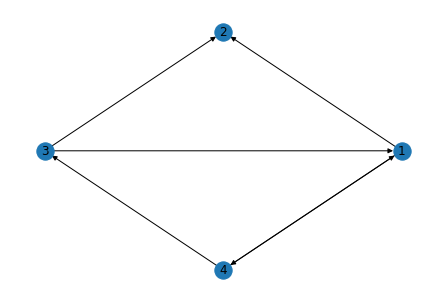
Digraphs¶

A directed graph or digraph is a graph where the edges have direction. The edge, often called an arrow, \((x,y)\) starts at node \(x\) and goes to node \(y\).

D = DiGraph()
D.add_edges_from([(1,2),(3,2),(4,3),(4,1),(1,4),(3,1)])
nx.draw(D, pos=nx.circular_layout(D), with_labels=True)

A node \(x\) in a digraph \(D\) has two neighborhoods, the out-neighborhood and the in-neighborhood. The out-neighborhood contains all the nodes \(y\) such that \(D\) contains the arrow \((x,y)\). The in-neighborhood of \(x\) contains all the nodes \(w\) such that \(D\) contains the arrow \((w,x)\). Thus every node will also have an out-degree and an in-degree.

It is easy to get the out-neighborhood of a node in a NetworkX digraph.

D[1]

AtlasView({2: {}, 4: {}})

The out-degree and in-degree can be obtained using the methods out_degree and in_degree respectively.

D.out_degree(3),D.in_degree(3)

(2,1)

Multigraphs¶

A multigraph is a graph that can have multiples edges connecting the same two nodes.

M = nx.MultiGraph()
M.add_edges_from([(1,2),(2,3),(3,1),(3,1),(3,1),(2,4),(2,4)])

Multigraphs also allow for edges to start and stop at the same node.

M.add_edge(1,1)

The neighborhood and degree are defined the same way as for graphs.

M[1]

AdjacencyView({2: {0: {}}, 3: {0: {}, 1: {}, 2: {}}, 1: {0: {}}})

M.degree(1)

6